I have had “The Beauty of Mathematics” for some time now, and as a book I’ve been reading during my leisure time, it has indeed piqued my interest a great deal. Since I don’t allocate much time to reading, averaging only one or two chapters a day, I finished all the chapters yesterday and was left wanting more.
From the title, it’s clear that this book is about mathematics, but it discusses the mathematical principles in practical applications (not involving specific implementations, just giving you an idea of what the principles are like). I never thought that the cosine theorem from middle school could have such great significance, along with Fermat’s theorem, etc. Dr. Wu Jun also explained artificial neural networks in very simple terms, indicating they have no relation at all (haha). I was dazzled by many ideas in the book; indeed, only scientific research can be the crystallization of human wisdom (I have long given up on those miscellaneous books).
This book does not discuss any methods for learning mathematics (it is by no means a learning guide) and falls under the category of popular science books. Finishing it will definitely spark your interest in mathematics (Trust me)!
Since I am not very good at math, I often consulted Wikipedia while reading, and I added links and footnotes to the mathematical concepts mentioned in the text.
Alright, enough with the preamble. Let’s get into the details.
Due to excessive length, I will only give one example (actually, I am just being lazy; if you want details, go buy the book). Let’s look at the practical applications of mathematics in computing.
Dr. Wu Jun spent a significant portion of “The Beauty of Mathematics” discussing natural language processing content (statistical language models, word segmentation, hidden Markov models, measures of information, etc.).
Natural language has gradually evolved from its inception into a way of expressing and conveying contextually-related information. Thus, for computers to process natural language, a fundamental issue is to establish a mathematical model that accommodates the contextual characteristics of natural language. This mathematical model is commonly referred to as the statistical language model (Statistical Language Model) in natural language processing.
Due to length, I won’t elaborate further, but just mention the bigram model of statistical language (of course, if a word’s probability is determined by the previous N-1 words, the model is called an N-gram model):
Assume S is a meaningful sentence composed of a specific sequence of words $w_1,w_2,w_3,…,w_n$, where n is the length of S. Now, we want to calculate the probability of S appearing in the text, which is mathematically referred to as the probability of S, $P(S)$. Since $S=w_1,w_2,w_3,…,w_n$, we can expand $P(S)$ thus:
$$P(S)=P(w_1,w_2,w_3,…,w_n)$$
Using the conditional probability formula, the probability of the sequence S appearing is equal to the product of the probabilities of each word appearing; thus, $P(S)$ can be expanded as:
$$P(S)=P(w_1)·P(w_2|w_1)·P(w_3|w_1,w_2)···P(w_n|w_1,w_2…w_{n-1})$$
However, we now face a problem — the computational load is too large, because the probability of each word appearing is akin to a dictionary. The first word $P(w_1)$ is straightforward to calculate, and the second word $P(w_2|w_1)$ is also not too difficult, but as mentioned, the possibilities for each word are as vast as a language dictionary. By the time we get to the last word, the conditional probability $P(S)=P(w_1,w_2,…,w_n)$ could be too numerous to estimate.
Fortunately, the Russian mathematician Markov proposed a concept:
Assume that the probability of any word $w_i$ appearing depends only on the preceding word $w_{i-1}$. This assumption is called the Markov assumption.
$$P(S)=P(w_1)·P(w_2|w_1)·P(w_3|w_2)···P(w_i|w_{i-1})···P(w_n|w_{n-1})$$
According to the definition of conditional probability, we can estimate the conditional probability $P(w_i|w_{i-1})$:
$$P(w_i|w_{i-1})=\frac{P(w_{i-1},w_i)}{P(w_{i-1})}$$
Estimating joint probabilities and marginal probabilities becomes very simple; we just need to use a corpus to count how many times the pair of words $w_{i-1},w_i$ appeared adjacent in the statistical text $*(w_{i-1},w_i)$ and how many times $w_{i-1}$ itself appeared in the same corpus $*(w_{i-1})$. Then, we can get the relative frequency of these words or bigrams by dividing these two counts by the size of the corpus $*$:
$$f(w_{i-1},w_i)=\frac{*(w_{i-1},w_i)}{*}$$
$$f(w_{i-1})=\frac{*(w_{i-1})}{*}$$
According to the law of large numbers, as long as the sample size is sufficient, the relative frequency equals the frequency, i.e.,
$$P(w_i,w_{i-1})\approx\frac{*(w_i,w_{i-1})}{*}$$
$$P(w_{i-1})\approx\frac{*(w_{i-1})}{*}$$
The value of $P(w_i|w_{i-1})$ is just the ratio of these two quantities, and since they share the same denominator, it can be eliminated:
$$P(w_i|w_{i-1})\approx\frac{*(w_i,w_{i-1})}{*(w_{i-1})}$$
OK, finally done. As you can see, using mathematics, we can simplify complex issues down to something this straightforward. Such a simple mathematical model can solve complex functions like speech recognition and machine translation; can we still call it the “uselessness of mathematics”?
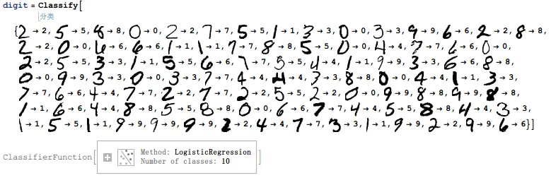
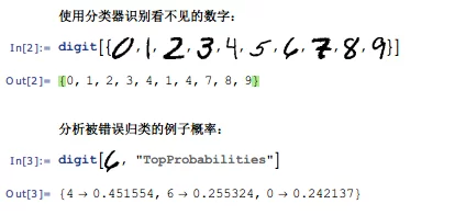
Once the model is established, training for the model (obtaining all the conditional probabilities in the model) is also essential. Recently, I discovered that Mathematica offers Classify, so I casually tried (faked) it out (unrelated to the model in the text).
- Conditional probability (English: conditional probability) refers to the probability of event A occurring given that another event B has already occurred. Conditional probability is denoted as P(A|B), read as “the probability of A given B.”
- Joint probability indicates the probability of two events occurring together. The joint probability of A and B is denoted as $P(A \cap B)$ or $P(A,B)$.
- Marginal probability is the probability of a particular event occurring. Marginal probability is derived as follows: in joint probability, merge those unnecessary events in the final result to obtain the total probability of the event, resulting in disappearance (apply summation for discrete random variables to get the total probability, apply integration for continuous random variables). This process is called marginalization. The marginal probability of A is denoted as $P(A)$, and the marginal probability of B is denoted as P(B).
- The law of large numbers, also known as the law of large numbers, describes the outcomes of repeated experiments over a significant number of trials. According to this law, the larger the sample size, the closer the average will be to the expected value.